8. Individual Risk, Insurance and Complete Markets
Learning objectives:
Risk and Complete Markets
General (Competitive) Equilibrium under complete asset markets:
- Representative agent result
Foundation for:
- arbitrage-free asset pricing models in Finance, and
- applied equilibrium models of the business cycle (a.k.a. Dynamic Stochastic General Equilibrium models)
- international trade and finance
Point of departure for models of incomplete markets and heterogeneous agents
8.1. Reading List
Minimal reading:
- LS, 8; or
- Mi, 13
Further reading:
- Debreu [De1959]
| [De1959] | (1, 2) Debreu, Gerard: Theory of Value, 1959, Wiley Publishers, New York. |
8.2. Introduction
Previously we focused on methods to help us solve dynamic stochastic optimization problems. The examples we encountered were mostly a single planner’s problem deciding on aggregate outcomes or a single partial equilibrium consumer’s problem. We will revisit the idea of decentralizing the process of allocating resources. Recall we have seen this before in the setting of the deterministic optimal growth model. Let’s take our insights from there, but now, we will study the structure of competitive general equilibrium in a dynamic and stochastic environment.
A first attempt to grasp the idea is to focus on exchange economies where resources are not produced but are pure endowments. You would have encountered simple endowment exchange economies, and in fact, studied competitive equilibria in your undergraduate microeconomics courses using the apparatus of the Edgeworth Box. In this course, we will work with more general setups with a finite set of traders/consumers and endowments follow some stochastic process. So if you keep your basic Edgeworth box training in mind, not much will be new here (except the countable time dimension, nature’s randomization on endowment streams and alternative Walrasian market structures with respect to time).
Why do we study these fake economies? As we will see towards the end of this chapter, the framework here can be further generalized and applied to a wide variety of problems. For example we can build dynamic stochastic (and general equilibrium) economies with optimizing agents useful for understanding asset pricing, consumption behavior, analyzing different government policies (fiscal and monetary), and even international macroeconomic problems like current account and exchange rate dynamics. Furthermore, the complete markets ideal will often be taken as a point of reference by and departure for alternative and quantitatively more plausible theories of incomplete asset markets. [1] These more complicated problems will appear in a more advanced course.
8.3. Timing and market structure
Gerard Debreu [De1959] provided the insight, in his Theory of Value, that a commodity can be thought of as indexed by date, location and state of nature. An economic equilibrium can then be thought of as all trades taking place at the beginning of time for the future delivery of goods contingent on the date and state of the world. To be able to obtain the promised delivery of such goods, traders at time \(0\) must be able to hold a piece of “contract” that entitles them to those goods when and if the future state occurs. Such contracts in Debreu’s world are called Arrow-Debreu securities.
Arguably, Debreu’s assumption on market structure is somewhat artificial. We all observe trades happening on a daily basis, or even minute by minute in some markets. We will consider an alternative market structure which delivers what is called a Radner equilibrium. This is an equilibrium where trade occurs sequentially with one-period Arrow securities that span all possible future states of nature. That is, for each current realized history of outcomes, all traders care about is a complete set of contracts that they can write with each other to promise the delivery of state-contingent consumption goods in the next period.
It turns out there is a nice equivalence result between the two market structures. They turn out to give identical consumption allocations. Furthermore, under the usual neoclassical assumptions, it turns out that allocations from either decentralized market structures are identical to the utilitarian social planner’s allocation. This suggests to us that if we restrict the process for endowments to be Markov, we can use recursive methods (dynamic programming) to solve the social planner’s allocation first, and then back out the competitive equilibrium relative prices implied by those allocations. However, this may not be possible when markets are imperfect or incomplete because the decentralized competitive equilibrium allocations will differ from the social planner’s.
We should also note early on that the complete markets model opens the way to further alternatives which we have no time to cover here. One can consider situations where it may be impossible for agents to write contracts for all possible contingencies. This is the world of incomplete asset markets. Alternatively, there may be markets with imperfect information, incomplete information or imperfect enforcement of agreements. Again, this will force contracts to be endogenously incomplete, so that agents cannot insure away all their idiosyncratic consumption risks.
8.4. Notion of an equilibrium
What do we mean by equilibrium, in general? We can think of an equilibrium as a “mapping” from the physical environment (preference, technology, information sets and market structure) to real allocations, such that
- agents optimize (they select their best actions),
- agents actions are consistent with each other’s actions, and
- the allocations are feasible.
An example of such an (economic) equilibrium concept is the Walrasian, or valuation equilibrium. Typically we want to show such equilibria exist and are unique. In some cases, an equilibrium need not be efficient or Pareto optimal. Recall the usual textbook discussions on inefficient equilibria when there exist externalities, information distortions or incentive problems.
8.5. Preferences and endowments
We first describe the setting for the infinite-horizon stochastic exchange economy with arbitrary (finite-state-space) stochastic endowment processes. We have the following objects:
Stochastic event \(s_{t}\in S = \{ s_{1},...,s_{n} \}\) for \(t \in \mathbb{N}\).
Publicly observable history of events up to and including \(t\): \(h^{t}=\left(s_{0},s_{1},...,s_{t}\right) \in S^{t}\), where \(S^{t}\) is the \(t\)-fold Cartesian product of \(S\).
Unconditional probability of observing history \(h^{t}\) is given by the probability measure \(\pi _{t}\left( h^{t}\right)\). Assume \(\pi \left(s_{0}\right) =1\).
Probability of observing \(h^{t}\) conditional on realization of \(h^{\tau}\) is \(\pi \left( h^{t}|h^{\tau}\right)\) for any \(t \geq \tau\).
\(I\) agents indexed by \(i=1,...,I\).
Agent \(i\) ’s
endowment of one good \(y_{t}^{i}\left( h^{t}\right)\) is some function of history of stochastic events, \(h^{t}\);
purchase of history-dependent consumption plan, \(c^{i}=\left\{ c_{t}^{i}\left(h^{t}\right) \right\} _{t=0}^{\infty }\) for each \(h^{t}\);
consumption plans are ordered by von Neumann-Morgernstern preferences
\[U\left( c^{i}\right) =\mathbb{E}_{0}\sum_{t=0}^{\infty }\beta ^{t}u\left( c_{t}^{i}\left( h^{t}\right) \right) =\sum_{t=0}^{\infty }\sum_{h^{t}}\beta ^{t}u\left( c_{t}^{i}\left( h^{t}\right) \right) \pi _{t}\left( h^{t}\right)\]where \(u^{\prime }\left( c\right) >0,u^{\prime \prime }\left( c\right) <0\) and \(\lim_{c\searrow 0}u^{\prime }\left( c\right) =+\infty\) (to ensure \(c_{t}>0\) for all \(t\)).
Note that \(\pi _{t}\left( h^{t}\right)\) can, for example, be induced by a Markov process. For now we don’t need to make this restriction, so we will keep track of all \(t\)-histories, \(h^{t}\).
Aggregate consumption in each period must not exceed aggregate endowment, for all possible paths of history. A feasible allocation must satisfy
for all \(t\) and for all \(h^{t}\).
8.7. Arrow-Debreu competitive equilibrium
Now we decentralize the economy to let markets decide on the allocations. How are the markets structured with respect to time? We begin with our first of two market structure assumptions. This is a version of Walrasian equilibrium where markets open for trade only once – all trades happen at the beginning of time, time \(0\), after \(s_{0}\) is known. At \(t=0\) agents exchange claims on time \(t\) consumption contingent on history \(h^{t}\) at price \(q_{t}^{0}\left( h^{t}\right)\). So there is a complete set of securities for all possible histories \(h^{t}\). After time \(0\) trades agreed to at \(t=0\) are executed no more trades occur after \(t=0\).
This implies that each agent faces only one budget constraint accounting for all trades across time and possible histories. Also it is assumed that agents honor all (forward) contracts so that all commodities are delivered contingent on date and event.
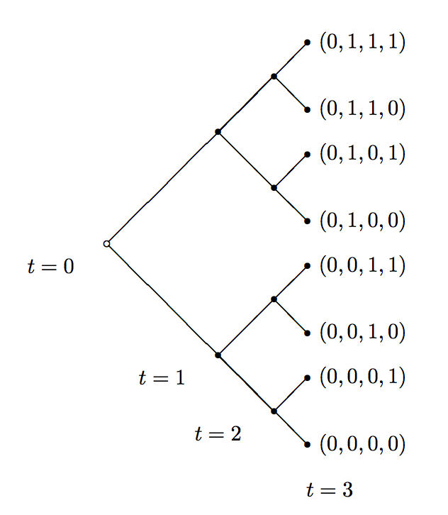
ADE Timing and Markets
Example
This example, borrowed from LS, is for \(S = \{0,1\}\) and shows a set of histories \(h^{t}\) up to \(t=3\). Consider consumer \(1\) whose endowments are such that \(y_{H} > y_{L}\) and
If the partial history were to be \(h^{3} = (s_{0},s_{1},s_{2},s_{3})= (0,1,0,1)\), then at time \(t=0\) this consumer can trade in a set of Arrow-Debreu securities that includes the one specifically for this possible history. (See Figure ADE Timing and Markets.)
That is, one which ensures a payout of some consumption for \(t=1\) and \(t=3\), when his endowment is low, and conversely the same consumer will deliver some consumption to someone else in \(t=0\) and \(t=2\).
In the Arrow-Debreu economy, each agent \(i \in \{1,...,I\}\) solves
subject to
where \(q_{t}^{0}\left( h^{t}\right)\) is the relative price, determined at time \(0\), of time \(t\) consumption good which is if history \(h^{t}\) is to be realized at \(t\). What is the price relative to? We have let one good be the numeraire good (more on this later).
The optimal choice of each agent \(i\) is characterized by the first-order conditions:
for each \(t \geq 0\) and \(h^{t} \in S^{t}\). Notice that \(\mu ^{i}\) is agent \(i\) ’s time-independent Lagrange multiplier on their time-0 intertemporal budget constraint.
Definition [Arrow-Debreu equilibrium]
A competitive equilibrium is a feasible allocation \(\left\{ c_{t}^{i}\left( h^{t}\right)\right\} _{t=0}^{\infty }\) and a price system \(\left\{ q_{t}^{0}\left(h^{t}\right) \right\} _{t=0}^{\infty }\) that solves each agent’s problem; i.e. it satisfies (6), (7), and \(\sum_{i=1}^{I}c_{t}^{i}\left( h^{t}\right) = \sum_{i=1}^{I}y_{t}^{i}\left( h^{t}\right)\) for all \(i=1,...,I\), and for all possible histories \(h^{t}\).
Notice that FONC Arrow-Debreu equilibrium] implies
for all \(i,j=1,...,I\). Using this and the (binding) feasibility constraint
we have
which looks just like (4) in the Pareto problem. Thus, \(c_{t}^{j}\left( h^{t}\right)\) depends only on current realized aggregate endowment, for all \(j=1,...,I\). This brings us to the following conclusion.
Proposition
The Arrow-Debreu competitive equilibrium allocation is a function of the realized aggregate endowment and does not depend on
- the particular history \(h^{t}\) leading up to that outcome, nor
- the realization of individual endowments
so that if \(h^{t} \neq h^{\tau}\) are such that \(\sum_{j}y_{t}^{j}\left(h^{t}\right) =\sum_{j}y_{\tau }^{j}\left( h^{\tau}\right)\) then \(c_{t}^{i}\left( h^{t}\right) = c_{\tau }^{i}\left( h^{\tau}\right)\).
Proposition [First fundamental welfare theorem]
The competitive equilibrium is a particular Pareto optimal allocation, where \(\mu _{i}=\lambda _{i}^{-1}\) for all \(i=1,...,I\), is unique (up to a multiplication by a positive scalar). Furthermore, the shadow prices for the planner \(\theta _{t}\left(h^{t}\right)\) are equal to Arrow-Debreu equilibrium price \(q_{t}^{0}\left( h^{t}\right)\).
8.7.1. Computing a competitive equilibrium
The following recipe provides a way to calculate the competitive equilibrium.
Negishi Algorithm
- Fix a value for one \(\mu _{i}\). E.g. set \(\mu _{1}=\mu >0\). Guess remaining \(\mu _{-i}\). Solve (8) and (9) for a candidate allocation \(\left\{ c_{t}^{i}\left( h^{t}\right) \right\}_{t=0}^{\infty }\) for all \(i=1,...,I\).
- Use (6) to solve for supporting price system \(q_{t}^{0}\left( h^{t}\right)\).
- Check budget constraint (7) for \(i=1,...,I\). For each \(i\) where LHS \(>(<)\) RHS, raise (lower) \(\mu _{i}\).
- Repeat 1-3 until convergence.
8.7.2. Equilibrium relative price system
Note the equilibrium price system \(\{q_{t}^{0}\left( h^{t}\right)\}_{t=0}^{\infty}\) is a function of equilibrium allocations \(\left\{ c_{t}^{i}\left( h^{t}\right) \right\} _{t=0}^{\infty }\) for all \(i=1,...,I\), given by (6) and has arbitrary units. Therefore \(q_{t}^{0}\left( h^{t}\right)\) can be normalized such that \(q_{0}^{0}\left( s_{0}\right) =1\), so the price system is relative to time \(0\) goods. This also implies, by (6), that the Lagrange multiplier for consumer \(i\) is just the marginal utility of time-\(0\) consumption, \(\mu _{i}=u^{\prime }\left( c_{0}^{i}\left( s_{0}\right) \right)\).
8.7.3. Asset-pricing implications
The benchmark asset pricing theory assumes complete markets. The price of an asset then represents the sum of prices (in time-0 terms) of a sequence of history-contingent claims. As we have seen, the time-\(t\) history \(h^{t}\)-contingent claim on consumption has a price \(q_{t}^{0}\left( h^{t}\right)\). An asset in a complete markets world is redundant because it merely synthesizes or replicates a bundle of history-contingent, dated claims, each of which is already priced by the Arrow-Debreu securities market.
8.7.3.1. Pricing redundant assets
Suppose the claim on consumption contingent on the realization of time \(t\) and history \(h^{t}\) is given by \(d_{t}\left( h^{t}\right)\) such that
We can think of \(d_{t}\left( h^{t}\right)\) as the contract or piece of paper that enables to holder to claim delivery of one unit of consumption if at time \(t\) the history were to be \(h^{t} = \tilde{h}^{t}\). Now, the price of that unit of consumption under history \(h^{t}\) is just \(q_{t}^{0}\left( h^{t}\right)\).
The stream of claims on consumption contingent on realization of time \(t\) and history \(h^{t}\) is \(\left\{ d_{t}\left( h^{t}\right) \right\} _{t=0}^{\infty }.\) Therefore, the price of any asset at time \(0\) that can replicate this stream of contingent claims has to be
Otherwise, someone else can construct another asset, by buying/selling history-contingent dated goods, such that the asset would replicate the desired stream of claims and make unlimited profits. This is called a no-arbitrage condition.
Definition
A riskless consol is an asset that provides one unit of consumption for sure, for all \(t\) and all \(h^{t}\). That is, \(d_{t}\left(h^{t}\right) =1\) for all \(t\), and all \(h^{t}.\) Price of riskless consol is
Definition
A riskless strip is a sequence of strips of payoffs on the riskless consol. Time \(\tau\) strip is just
Price in time 0 terms: \(\sum_{h^{t}}q_{t}^{0}\left( h^{t}\right) .\)
8.7.3.2. Pricing tail assets
Suppose we have an investor who wishes to know what the price of an asset that entitles her to a stream of dividends starting from some future date \(\tau \geq t \geq 1\) is. What is the time 0 price of the dividend stream \(\left\{ d_{\tau}\left( h^{\tau}\right) \right\} _{\tau \geq t }\)? To calculate this we strip off first \(t -1\) periods of dividends and start calculating from time \(t\).
Time \(0\) price of an asset that pays dividend stream \(\left\{ d_{\tau}\left( h^{\tau}\right) \right\} _{\tau \geq t }\), if \(h^{t}\) is realized:
Note that summing over \(h^{\tau}| h^{t}\) means summing over all possible histories \(h^{\tau}\) which could have been generated by the given history up to time \(t\): \(\widetilde{h}^{t}=h^{t}.\)
Recall FONC for agent \(i\) in (6):
So we can write the state price deflator in time \(t \leq \tau\) terms, for all agents \(i\), as
This equation says that the price of time \(\tau\) delivery, history \(h^{\tau}\)-contingent consumption, relative to the price of time \(t \leq \tau\) delivery, history \(h^{t }\)-contingent consumption is equal to the marginal rate of substitution of consumption across \(\tau\) and \(t\), taking into account the probability that state \(h^{\tau}\) is realized, given realization of \(h^{t }\).
So the price at \(t\) of the tail asset is
where numeraire is time \(t\), history \(h^{t}\), consumption good, or \(% q_{t}^{t}\left( h^{t}\right) =1\). This says that an asset (e.g. equity) bought at time \(t\) entitles buyer/owner to dividends from \(t \geq 1\) onward.
This notation, or re-basing the numeraire to history-\(h^{t}\) good can also be interpreted as re-opening the Arrow-Debreu market at time \(t\) under history \(h^{t}\). It can be shown that all individuals will not deviate from their original consumption plan at time 0 even markets re-open at time \(t\) under history \(h^{t}\).
8.7.3.3. Pricing one-period returns
The one-period version of the state price deflator (10) is
So the price, at time \(\tau\) history \(h^{\tau }\), of a claim to a random payoff \(\omega \left( s_{\tau +1}\right)\) will be
for all \(i \in \{1,...,I\}\).
Dividing through on both sides, we get
\(R_{\tau +1}:= \omega \left( s_{\tau +1}\right)/p_{\tau}^{\tau}(h^{\tau})\) is the one-period gross return on the asset. and \(m_{\tau +1}=\beta u^{\prime }\left( c_{\tau+1}^{i}\right) /u^{\prime }\left( c_{\tau }^{i}\right)\) is called a stochastic discount factor on this return. Both are random variables whose expected values are with respect to the distribution of \(s_{\tau + 1}\) conditional on \(h^{\tau}\). This is just a stochastic Euler equation relating optimal risky intertemporal consumption allocations to asset returns!
8.8. Sequential markets and Arrow securities
Now we consider the alternative assumption on market structure. It will turn out that consumption allocations in this economy is identical to the Arrow-Debreu economy’s. This is because the key asset pricing relationship in ([LSapeqn]) can be reproduced from this economy with sequential trades in one-period ahead Arrow securities.
In this market trading structure, we have the following assumptions:
- Trade occurs at each \(t\geq 0\).
- Trade in one-period complete Arrow securities. At each \(t\) reached with history \(h^{t}\), traders meet to trade for history \(h^{t+1}\)-contingent goods deliverable in \(t+1\).

SME Timing and Markets
Example
Figure SME Timing and Markets depicts another example from for a sequential trading economy where \(S = \{0,1\}\). At \(t=2\), trades occurs for only \(t=3\) goods at states that can be reached from the realized \(t=2\) history, \(h^{2}=(0,1,1)\).
There are two building blocks we need to consider first when moving from the Arrow-Debreu economy to one when there are sequential trades in one-period Arrow securities. The first has to do with using wealth as a state variable. The second is a restriction that prevents forever-borrowing schemes by agents.
8.8.1. A state variable in the sequential economy
First, we need to find an appropriate individual state variable in each period for each consumer to be able to base his trading decisions for his next-period contingent claims on consumption. This state variable will serve to provide the right choices of consumption each period so that there will be enough resources left for trades on future contingent claims on consumption. It turns out that this state variable is the present value (in terms of history \(h^{t}\) and date \(t\)) of all expected current and future net claims, which represents the current wealth of the consumer.
Let’s recall the setting from the Arrow-Debreu economy. Specifically, at time \(t\) agent \(i\)’s net claim to delivery of goods in some future period \(\tau \geq t\) under history \(\widetilde{h}^{\tau}\) contingent on the realization \(\widetilde{h}^{t}=h^{t}\) is
Agent \(i\)’s wealth at time-\(t\) is just the time-\(t\) expected value of all her current and future net claims conditional on time-\(t\), history \(h^{t}\):
This has the same expression as the value of a tail asset!
Since in any period, aggregate (across all \(i\)’s) endowment must equal aggregate consumption – i.e. the feasibility constraint (1) implies
for all \(t\) and all \(h^{t}\). This is just implies that the cross-sectional distribution of tail wealth across all agents \(i\) sums to zero, since all contingent debt sellers are balanced out by buyers. When we move from this Arrow-Debreu world to the sequential markets world, we can relate this tail wealth of each \(i\), \(\Omega_{t}^{i}\left( h^{t}\right)\), to the time \(t\) history \(h^{t}\) individual asset of the sequential markets world.
8.8.2. Debt limits
In the Arrow-Debreu economy, households face a single intertemporal budget constraint that ensures intertemporal solvency. In the sequential markets setting, there will be a sequence of budget constraints. We need to ensure that sequential asset trades are not open to “Ponzi schemes” – i.e. consumers cannot forever be in the position of consuming more than their endowments each period. [2]
We will consider the weakest possible restrictions called natural debt limits. The requirement is that it must be feasible for the consumer to repay his state contingent debt in every possible state. So what does this limit look like?
Definition [Natural debt limit]
Let the Arrow-Debreu price in terms of the time \(t\) history \(h^{t}\) numeraire good be \(q_{\tau }^{t}\left( h^{\tau}\right)\) for \(\tau \geq t\). The value of the tail of \(i\)’s endowment sequence at time \(t\) given history \(h^{t}\) is
is the natural debt limit at time \(t\) and history \(h^{t}\).
The maximal amount that \(i\) can repay his debt starting from time \(t\) is thus the expected tail value of his endowment starting out from time \(t\) given history \(h^{t}\). Alternatively, this says the most \(i\) can do is to consume zero forever sarting from time \(t\) to repay existing debt at time \(t\) history \(h^{t}\). At each time \(t\), \(i\) will face one such borrowing constraint for each possible realization \(h^{t+1}\) the next period.
8.8.3. Sequential trading
We will now use variables with the decoration “tilde” on top to distinguish prices and allocations in sequential trading markets from the Arrow-Debreu time \(0\) market.
Markets are open for trade in one period-ahead state-contingent claims every period. Every agent trades claims, each period \(t\geq 0\), to \(t+1\), \(h^{t+1}\)-contingent consumption. So each period \(t\), with history \(h^{t},\) an agent \(i\) can
- bring into it a contingent claim \(\widetilde{a}_{t}^{i}\left( h^{t}\right)\) to time \(t\) consumption, and/or
- consume time \(t\) consumption using time \(t\) endowment \(y\left( h^{t}\right) .\)
Suppose the pricing kernel \(\widetilde{Q}_{t}\left( s_{t+1}|h^{t}\right)\) exists. This is the price of one unit of time \(t+1\) consumption, contingent on realization of \(s_{t+1}\) in \(t+1\), given history leading up to time \(t\) is \(h^{t}.\) Agent \(i\)’s sequence of budget constraints must be
for \(t\geq 0\), at each \(h^{t}\).
Note at time \(t\), \(i\) chooses \(\widetilde{c}_{t}^{i}\left( h^{t}\right)\) and chooses a vector \(\left\{ \widetilde{a}_{t+1}^{i}\left(s_{t+1},h^{t}\right) \right\}\) that has the same number of elements as the possible states \(s_{t+1}\) given \(h^{t}\).
The no-Ponzi scheme constraint for all possible states is
Agent \(i\) solves
for given initial wealth \(\widetilde{a}_{0}^{i}\left( h^{0}\right)\).
The first-order necessary condition for a maximum is
for all \(s_{t+1}\), \(t\geq 0\) and \(h^{t}\). In the optimal solution, the no-Ponzi scheme constraint does not bind, \(\nu _{t}^{i}\left( h^{t};s_{t+1}\right) =0\), for all states and dates. Why? The Inada condition on period utility implies consumption is strictly positive. If the constraint binds, consumption from \(t+1\) has to be zero forever by the natural debt limit, which implies that the consumer has infinite marginal utility of consumption. But agents can do better by re-allocating earlier consumption to later periods after the constraint binds, to relax it.
Since \(\nu _{t}^{i}\left( h^{t};s_{t+1}\right) =0\), for all states and dates, the first-order conditions reduce to
for all \(s_{t+1}\), \(t\geq 0\) and \(h^{t}\). This is a familiar looking one-period pricing kernel we encountered in the Arrow-Debreu economy! So this is telling us that we’re on to something.
Definition
A distribution of wealth is a vector \(\overrightarrow{\widetilde{a}}_{t}\left( h^{t}\right) =\left\{ \widetilde{a}_{t}^{i}\left( h^{t}\right) \right\} _{i=1}^{I}\) satisfying \(\sum_{i}\widetilde{a}_{t}^{i}\left( h^{t}\right) =0.\)
Definition
A sequential trading competitive equilibrium is an initial distribution of wealth \(\overrightarrow{\widetilde{a}}_{0}\left( s_{0}\right)\), an allocation (sequence of allocations for all agents) \(\left\{ \widetilde{c}^{i}\right\} _{i=1}^{I}\) and pricing kernels \(\widetilde{Q}_{t}\left( s_{t+1}|h^{t}\right)\) such that
- for all \(i\), given \(\widetilde{a}_{0}^{i}\left( s_{0}\right)\) and \(% \widetilde{Q}_{t}\left( s_{t+1}|h^{t}\right)\), the consumption allocation \(\widetilde{c}^{i}=\left\{ \widetilde{c}_{t}^{i}\right\} _{t=0}^{\infty }\) solves agent \(i\)’s optimization problem;
- for all realizations of \(\left\{ h^{t}\right\} _{t=0}^{\infty }\) the agent’s consumption allocation \(\widetilde{c}^{i}\) and implied asset portfolios \(\left\{ \widetilde{c}_{t}^{i}\left( h^{t}\right) ,\left\{ \widetilde{a}_{t+1}^{i}\left( s_{t+1},h^{t}\right) \right\} _{s_{t+1}}\right\} _{i}\) satisfy \(\sum_{i}\widetilde{c}_{t}^{i}\left( h^{t}\right) =\sum_{i}y_{t}^{i}\left( h^{t}\right)\) and \(\sum_{i}\widetilde{% a}_{t+1}^{i}\left( s_{t+1},h^{t}\right) =0\) for all \(s_{t+1}\).
What is the initial distribution of wealth \(\overrightarrow{\widetilde{a}}% _{0}\left( s_{0}\right)\)? In the Arrow-Debreu world, time-0 trading determines a particular \(% \overrightarrow{\widetilde{a}}_{0}\left( s_{0}\right).\) So with an appropriate choice of initial wealth distribution, we can show that there is an equivalence in real allocations under the Arrow-Debreu world and under the sequential markets world.
8.8.4. Equivalence in equilibrium allocations
Now we are ready to show that the two economies’ allocations are equivalent when markets are complete.
Proposition
The time-0 trading arrangement in the Arrow-Debreu equilibrium with complete markets has the same allocations as the sequential trading arrangement with one-period complete Arrow securities, i.e. \(\left\{ c^{i}\right\} _{i=1}^{I}=\left\{ \widetilde{c}^{i}\right\} _{i=1}^{I}\), for an appropriate initial distribution of wealth in the sequential markets equilibrium, \(\left\{ \widetilde{a}_{0}^{i}\left( s_{0}\right) \right\} _{i=1}^{I}\).
We provide an outline of a proof. First we show that we can construct the same allocations in the sequential markets equilibrium from the Arrow-Debreu equilibrium.
Take Arrow-Debreu equilibrium \(q_{t}^{0}\left( h^{t}\right)\) as given.
Suppose there exists \(\widetilde{Q}_{t}\left( s_{t+1}|h^{t}\right)\) satisfying recursion
\[\begin{split}\begin{aligned} q_{t+1}^{0}\left( h^{t+1}\right) &=\widetilde{Q}_{t}\left( s_{t+1}|h^{t}\right) q_{t}^{0}\left( h^{t}\right) \\ &\Leftrightarrow \widetilde{Q}_{t}\left( s_{t+1}|h^{t}\right) =\frac{% q_{t+1}^{0}\left( h^{t+1}\right) }{q_{t}^{0}\left( h^{t}\right) }% =q_{t+1}^{t}\left( h^{t+1}\right) .\end{aligned}\end{split}\]To show 2 is true, take Arrow-Debreu equilibrium first-order conditions from two succesive periods and write:
\[\beta \frac{u^{\prime }\left( c_{t+1}^{i}\left( h^{t+1}\right) \right) }{% u^{\prime }\left( c_{t}^{i}\left( h^{t}\right) \right) }\pi _{t}\left( h^{t+1}|h^{t}\right) =\frac{q_{t+1}^{0}\left( h^{t+1}\right) }{% q_{t}^{0}\left( h^{t}\right) }\]But then if 2 is true, it must be that
\[\begin{split}\begin{aligned} \beta \frac{u^{\prime }\left( c_{t+1}^{i}\left( h^{t+1}\right) \right) }{% u^{\prime }\left( c_{t}^{i}\left( h^{t}\right) \right) }\pi _{t}\left( h^{t+1}|h^{t}\right) &= \widetilde{Q}_{t}\left( s_{t+1}|h^{t}\right) \\ &=\beta \frac{u^{\prime }\left( \widetilde{c}_{t+1}^{i}\left( h^{t+1}\right) \right) }{u^{\prime }\left( \widetilde{c}_{t}^{i}\left( h^{t}\right) \right) }\pi _{t}\left( h^{t+1}|h^{t}\right) .\end{aligned}\end{split}\]So then, Arrow-Debreu equilibrium is equivalent to the sequential markets equilibrium in terms of allocations, \(\left\{ c^{i}\right\} _{i=1}^{I}=\left\{ \widetilde{c}^{i}\right\} _{i=1}^{I}\).
Next we show we can construct an Arrow-Debreu equilibrium allocation from the sequential markets equilibrium:
Need to pick initial wealth in the sequential markets equilibrium so that sequence of BCs in sequential markets equilibrium will be consistent with intertemporal BC for Arrow-Debreu equilibrium. Guess that \(\left\{ \widetilde{a}_{0}^{i}\left( s_{0}\right) \right\} _{i=1}^{I}=\mathbf{0}% _{I\times 1}\). Why? In Arrow-Debreu equilibrium, at time \(0\), agents bring in only their endowments, \(y_{0}\left( s_{0}\right)\). Good guess for sequential markets equilibrium too.
At \(t\geq 0\) and history \(h^{t}\), \(i\) chooses asset portfolio, \(% \widetilde{a}_{t+1}^{i}\left( s_{t+1},h^{t}\right) =\Omega _{t+1}^{i}\left( h^{t+1}\right)\) for all \(s_{t+1}.\) The expected value in date \(t\) terms is
\[\begin{split}\begin{aligned} \sum_{s_{t+1}}\widetilde{a}_{t+1}^{i}\left( s_{t+1},h^{t}\right) \widetilde{Q% }_{t}\left( s_{t+1}|h^{t}\right) &=\sum_{s_{t+1}}\Omega _{t+1}^{i}\left( h^{t+1}\right) q_{t+1}^{t}\left( h^{t+1}\right) \\ &=\sum_{\tau =t+1}^{\infty }\sum_{h^{\tau}|h^{t}}q_{\tau }^{t}\left( h^{\tau}\right) \left[ c_{\tau }^{i}\left( h^{\tau}\right) -y_{\tau }^{i}\left( h^{\tau}\right) \right]\end{aligned}\end{split}\]just the tail value of wealth!
Show that \(i\) can afford this portfolio strategy. Use sequence of sequential markets equilibrium BCs. At time \(0\) given \(\widetilde{a}_{0}^{i}\left( s_{0}\right) =0\),
\[\widetilde{c}_{0}^{i}\left( s_{0}\right) +\sum_{t=1}^{\infty }\sum_{h^{t}}q_{t}^{0}\left( s_{t}\right) \left[ c_{t}^{i}\left( h^{t}\right) -y_{t}^{i}\left( h^{t}\right) \right] =y_{0}^{i}\left( s_{0}\right) +0\]But this is the same as (5) in the Arrow-Debreu equilibrium. \(\Rightarrow\) \(\widetilde{c}_{0}^{i}\left( s_{0}\right) =c_{0}^{i}\left( s_{0}\right)\).
For all \(t>0\), we can write \(\widetilde{a}_{t}^{i}\left( h^{t}\right) =\Omega _{t}^{i}\left( h^{t}\right)\), and the time \(t\) BC is
\[\begin{split}\widetilde{c}_{t}^{i}\left( h^{t}\right) +\sum_{s_{t+1}}\widetilde{a}_{t+1}^{i}\left( s_{t+1},h^{t}\right) \widetilde{Q}_{t}\left(s_{t+1}|h^{t}\right) & = y_{t}^{i}\left( h^{t}\right) +\widetilde{a}% _{t}^{i}\left( h^{t}\right) \\ \Rightarrow \sum_{s_{t+1}}\widetilde{a}_{t+1}^{i}\left( s_{t+1},h^{t}\right) \widetilde{Q}_{t}\left( s_{t+1}|h^{t}\right) & =\Omega _{t}^{i}\left( h^{t}\right) -\left[ \widetilde{c}_{t}^{i}\left( h^{t}\right) -y_{t}^{i}\left( h^{t}\right) \right] \\ \Rightarrow \sum_{s_{t+1}}\Omega _{t+1}^{i}\left( h^{t+1}\right) q_{t+1}^{t}\left( h^{t+1}\right) & =\Omega _{t}^{i}\left( h^{t}\right) -\left[ \widetilde{c}_{t}^{i}\left( h^{t}\right) -y_{t}^{i}\left( h^{t}\right) % \right] \\ \Rightarrow \sum_{\tau =t+1}^{\infty }\sum_{h^{\tau}|h^{t}}q_{\tau }^{t}\left( h^{\tau}\right) \left[ c_{\tau }^{i}\left( h^{\tau}\right) -y_{\tau }^{i}\left( h^{\tau}\right) \right] & =\Omega _{t}^{i}\left( h^{t}\right) -\left[ \widetilde{c}_{t}^{i}\left( h^{t}\right) -y_{t}^{i}\left( h^{t}\right) \right]\end{split}\]It then follows from step 3 and the above that \(\widetilde{c}_{t}^{i}\left(h^{t}\right) =c_{t}^{i}\left( h^{t}\right)\) for all \(t\) and \(h^{t}\).
Note
The last step in 4 relies on the fact that agents \(i\) will not want to increase current consumption by reducing some component of the asset portfolio. Time consistency in their choice.
Specifically, The household needs to ensure that the plan \(\left\{ c_{\tau }^{i}\left( h^{\tau}\right) \right\}\) can be attained beginning next period for all states.
To do so, it must deduct the commitment to future consumption from the natural debt limit. That is
\[\begin{split}\begin{aligned} -\widetilde{a}_{t+1}^{i}\left( s_{t+1}\right) &\leq A_{t+1}^{i}\left( h^{t+1}\right) -\sum_{\tau =t+1}^{\infty }\sum_{h^{\tau}|h^{t+1}}q_{\tau }^{t+1}\left( h^{\tau}\right) c_{\tau }^{i}\left( h^{\tau}\right) \\ &= - \Omega _{t+1}^{i}\left( h^{t+1}\right) \\ \Rightarrow \widetilde{a}_{t+1}^{i}\left( s_{t+1}\right) & \geq \Omega _{t+1}^{i}\left( h^{t+1}\right)\end{aligned}\end{split}\]This prevents the household from increasing current consumption, thereby reducing next period wealth below \(\Omega _{t+1}^{i}\left( h^{t+1}\right)\) which would have violated the optimal plan supported by the pricing kernel
\[\widetilde{Q}_{t}\left( s_{t+1}|h^{t}\right) =\beta \frac{u^{\prime }\left( \widetilde{c}_{t+1}^{i}\left( h^{t+1}\right) \right) }{u^{\prime }\left( \widetilde{c}_{t}^{i}\left( h^{t}\right) \right) }\pi _{t}\left( h^{t+1}|h^{t}\right) .\]
8.8.5. Discussions
The equivalence between Arrow-Debreu equilibrium and Arrow’s sequential markets equilibrium follows from two key factors:
- Agents are v.N-M expected utility maximizers – their once-and-for-all time \(0\) choices are time consistent. Past actions affect future payoffs but future actions do not affect past payoffs.
- Under complete markets, the budget sets defined by the two formulations are equivalent, and thus Arrow-Debreu equilibrium prices of contingent claims are equal to Arrow’s spot prices weighted by the price in period 1 of the appropriate Arrow security.
The assumptions about the state variables so far in the Arrow-Debreu equilibrium and sequential markets equilibrium economies are too general to be useful – at each \(t\), state variables are made up of the entire history leading up to \(t\), i.e. \(h^{t}:=\left( s_{0},s_{1},...,s_{t}\right)\).
For practical purposes, we need to discipline the evolution of the state further – e.g. to be Markovian – so only a few state variables suffice to describe the position of the economy at each time period.
We’ll look at a recursive competitive equilibrium formulation of the sequential markets equilibrium and Arrow-Debreu equilibrium.
8.9. Recursive competititive equilibria
Previously, we have shown that the Arrow-Debreu equilibrium and sequential markets equilibrium have identical equilibrium allocations.
However, we had a rather general setup in terms of the stochastic process which generates history dependence in equilibrium allocations and prices. Specifically, the equilibrum allocation \(\left\{ c_{t}^{i}\left( s^{t}\right) \right\}_{t=0}^{\infty }\), pricing kernel \(Q_{t}\left( s_{t+1}|h^{t}\right)\) and wealth distributions \(a_{t}^{i}\left( h^{t}\right) _{i=1}^{I}\) depended on entire an history \(h^{t}=\left( s_{0},s_{1},s_{2},...,s_{t}\right)\). This is far to untractable for practical purposes.
We want to discipline the model further. We want to be able to store history in a small nutshell – a sufficient statistic or small number of state variables each period. To do this, restrict exogenous forcing processes to be Markov, so that we have a recursive representation of the sequential markets equilibrium.
8.9.1. Endowments with Markov property
Consider the state space, \(S\). The exogenous events that drive the endowment process is \(s\in S\). Let \(s\) be governed by a Markov chain:
- \(\pi _{0}\left( s\right) =\Pr \left( s_{0}=s\right)\).
- \(\pi \left( s^{\prime }|s\right) =\Pr \left( s_{t+1}=h^{\prime }|s_{t}=s\right).\)
The Markov chain induces a sequence of probability measures on histories \(h^{t}\). Recall our lessons from Markov chains. The probability of realizing history \(h^{t}\) is thus calculated as
where it is assumed \(\pi _{0}\left( s_{0}\right) =1\).
The Markov property says that
where \(\pi _{t}\left( h^{t}|h^{k}\right)\) depends only on state \(s_{k}\) at \(k<t\) and the history prior to \(k\) is redundant.
\(\pi _{3}\left( h^{3}|h^{2}\right) =\pi _{3}\left( \left( s_{0},s_{1},s_{2},s_{3}\right) |\left( s_{0},s_{1},s_{2}\right) \right) =\pi \left( s_{3}|s_{2}\right).\)
Then, for each \(i=1,...,I\), we can write endowments as
Since \(s_{t}\) is a Markov process, \(y_{t}^{i}\left( h^{t}\right)\) will also be a Markov process.
8.9.2. Equilibrium inherits Markov property
Recall under no restrictions on the exogenous stochastic process we had the following result: The Arrow-Debreu competitive equilibrium allocation is a function of the realized aggregate endowment and and does not depend on
- the particular history \(h^{t}\) leading up to that outcome, nor
- the realization of individual endowments
so that \(c_{t}^{i}\left( h^{t}\right) =c_{\tau }^{i}\left( h^{\tau }\right)\) for \(h^{t}\) and \(h^{\tau }\) \(\Leftrightarrow\) \(\sum_{j}y_{t}^{j}\left( h^{t}\right) =\sum_{j}y_{\tau }^{j}\left( h^{\tau }\right)\). With endowment possessing the Markov property, we further have allocations
and the pricing kernel in the sequential markets equilibrium
as functions of only the current state \(s_{t}.\) We can also show that Arrow-Debreu equilibrium price
is history-independent.
Given \(y_{t}^{i}\left( s^{t}\right)\) a Markov process, the Arrow-Debreu equilibrium price of date-\(\tau\) history \(h^{\tau}\) consumption goods in terms of date \(t\), \(0\leq t \leq \tau\), history \(h^{t}\) goods is not history dependent: \(q_{\tau}^{t}\left( h^{\tau}\right) =q_{j}^{k}\left( \widetilde{h}^{k}\right)\) for \(j,k\geq 0\) such that \(% \tau-t =k-j\) and \(\left( s_{t },s_{t +1},...,s_{\tau}\right) =\left( \widetilde{s}_{j},\widetilde{s}_{j+1},...,\widetilde{s}_{k}\right)\).
Natural debt limits and household wealth are also history independent: \(A_{t}^{i}\left( s^{t}\right) =A^{i}\left( s_{t}\right)\) and \(\Omega _{t}^{i}\left( s^{t}\right) =\Omega ^{i}\left( s_{t}\right)\). Each agent enters every period with wealth independent of past endowment realizations. Past trades have fully insured away all idiosyncratic endowment risks. So an agent enters the current period with current-state contingent wealth just sufficient to fund a trading scheme that insures against future idiosyncratic risks.
Here’s the invisible hand outcome. The pricing kernel \(Q\left( s_{t}|s_{t-1}\right)\) thus provides the correct signal, along with market clearing, to coordinate trade in time \(t-1\) such that all idiosyncratic risks are eliminated. However, if there are aggregate risks, they would still have to be borne by all agents.
8.9.3. Recursive formulation
With Markov endowment and given pricing kernel \(Q(s'|s)\), we can re-state the agents’ individual infinite-horizon expected utility maximization problems recursively. For agent \(i\), the Bellman equation is
subject to
Let the optimal decision rules associated with the fixed-point solution of the Bellman equation be
for each \(i = \{1,...,I\}\).
We can show that this optimal solution depends on the price kernel \(Q\left(s^{\prime }|s\right)\). Evaluate the first-order condition for the RHS of each Bellman equation and apply the Benveniste-Scheinkman formula to get
where \(c=h^{i}\left( a,s\right)\) and \(\widehat{a}\left( s^{\prime }\right) =g^{i}\left( a,s,s^{\prime }\right)\).
A recursive competitive equililibrium is an initial distribution of wealth \(\left\{ a_{0}^{i}\right\} _{i=1}^{I}\) a pricing kernel Q\(\left( s^{\prime }|s\right)\), sets of value functions \(\left\{v^{i}\left( a,s\right) \right\} _{i=1}^{I}\) and decision rules \(\left\{h^{i}\left( a,s\right) ,g^{i}\left( a,s,s^{\prime }\right) \right\} _{i=1}^{I}\) such that
- for all \(i\), given \(a_{0}^{i}\) and the pricing kernel, the decision rules solve the household \(i\)’s problem;
- for all histories \(\left\{ s_{t}\right\} _{t=0}^{\infty }\), the consumption and assets \(\{\{c_{t}^{i},\{\widehat{a}_{t+1}^{i}\left( s^{\prime }\right) \}_{s^{\prime }}\}_{i}\}_{t=0}^{\infty }\) implied by the decision rules satisfy \(\sum_{i}c_{t}^{i}=\sum_{i}y^{i}\left( s_{t}\right)\) and \(\sum_{i}\widehat{a}_{t+1}^{i}\left( s^{\prime }\right) =0\) for all \(t\) and \(s^{\prime }\).
8.10. Asset pricing with Markovian economies
We saw that when we assumed stochastic processes that are Markov, we could write down the competitive equilibrium characterization recursively. Specifically, wealth at each time period no longer depends of the entire history of endowment outcomes but only on the current state. This also allows us to price future state-contingent claims on consumption easily, without having to condition the prices on (possibly infinite) entire histories.
8.10.1. \(j\)-step ahead pricing kernel
Recall now, with a Markovian state for the economy, the one-step-ahead pricing kernel is \(Q(s'|s)\). This is the price of a contingent claim on a unit of consumption if some state \(s' \in S\) occurs next period, given the current-period state is some \(s \in S\). Let \(Q_{j}(s_{t+j}|s_{t}): = Q_{j}(s'|s)\) be the price of one unit of consumption if state \(s'\) occurs \(j \geq 1\) periods ahead from current period \(t\), given the current state is \(s\).
Since a complete set of markets exists for all \(j\) periods ahead contingent claims, a consumer \(i\), at the end of period \(t\), can always buy \(z_{t,j}^{i}(s_{t+j})\) units of contingent claims that promise to pay \(z_{t,j}^{i}(s_{t+j})\) units of consumption if state \(s_{t+j}\) is realized in period \(t+j\), for \(j \geq 1\). Recall that agent \(i\)’s sequential budget constraint is
The agent’s next period wealth depends on next period state \(s_{t+1}\) and the composition of the asset portfolio:
So the outcome \(s_{t+1}\) will determine which element of the \(n\)-dimensional vector
pays off at time \(t+1\). But this is only one component of time \(t+1\) wealth. The second term on the RHS, conditional of outcome \(s_{t+1}\) when time \(t+1\) arrives, is the expected payoffs (i.e. capital gains or losses) from holding longer term claims on \(t+1+j\), \(j \geq 1\), consumption. Together they make up next-period – i.e. \(t+1\) – wealth if \(s_{t+1} \in S\) is to be realized.
Using this fact, the sequence of budget constraints becomes
Note that the first-order condition for a optimal plan by agent \(i\) will imply that
(You should try working this out to check.) Since optimality also requires (11) holds, we then have
a recursive formula for computing \(j\)-step ahead pricing kernels for \(j = 2,3,...\).
8.10.2. Arbitrage-free pricing and redundant assets
Now we can relate the complete markets model to arbitrage-free pricing theory in finance. Specifically, any additional assets added to the agent’s portfolio of complete Arrow securities, is “redundant”. That is, the one-step ahead pricing kernel for Arrow securities must impose restrictions on the price of the redundant asset so that the agent’s budget set remains unaltered, if the agent is made to hold this asset. We will show this using just the sequence of budget constraints for an agent.
Let’s make this clear with the following tweak to our agent’s problem in the sequential markets model. Now we’re getting bored with the name “agent”. Let’s call him/her Sam. Suppose, apart from purchasing \(z_{t,j}(s_{t+j})\) units of \(j\)-step ahead complete Arrow securities, Sam also trades an ex-dividend stock called a Lucas tree. [2] A unit of this stock allows Sam to have the right to a unit of fruit or dividend \(d(s_{t+1})\) from this Lucas tree, if state \(s_{t+1}\) occurs. Sam can buy \(N_{t}\) units of this stock. The ex-divident price is \(p(s_{t})\). So Sam can obtain \(N_{t}[p(s_{t+1})+d(s_{t+1})]\) units of consumption in \(t+1\) if \(s_{t+1}\) occurs then. Again \(a_{t}\) is Sam’s wealth not including her endowment \(y(s_{t})\).
Now Sam’s budget constraint for any time \(t \in \mathbb{N}\) is
This just says that Sam can spend her net wealth at the end of \(t\) to purchase a portfolio of Arrow securities or a share in the Lucas tree. Recall that her budget constraint can also be written as
Now with the possibility of holding the stock apart from state-contingent claims, her next-period asset contingent on outcome \(s_{t+1} \in S\) must be
for \(t \in \mathbb{N}\). The present expected value of \(a_{t+1}(s_{t+1})\), conditional on \(s_{t}\), is just calculated as \(\sum_{s_{t+1}}Q_{1}(s_{t+1}|s_{t})a_{t+1}(s_{t+1})\). Multiply (15) by \(Q_{1}(s_{t+1}|s_{t})\) and sum over all \(s_{t+1} \in S\) and rearrange to get
Here’s the simple hack that says a lot. Substitute (16) into (13) to get the sequence of budget constraints as:
To be consistent with the budget constraint (14), the first two terms on the LHS must be equal to zero. Alternatively, if they are not zero, it mean the LHS (which makes up the expected present value of future assets) can be increased without bounds by buying/selling either the stock (first term) or the Arrow securities (second term), and thereby consumption can be increased without bounds. In equilibrium, such unbounded profit opportunities cannot be possible so we must have the two arbitrage-free pricing conditions
for all \(t \in \mathbb{N}\).
The first condition says that the price of the redundant stock must equal the expected present value of future stock price plus dividend payoffs. The second is the familiar recursive formula for computing a \(j\)-step pricing kernel for the contingent claims, and recall that this formula is consistent with (12) which has encoded the first-order condition for an optimal consumption plan by the agent.
8.11. Incomplete markets and asset pricing
What if we don’t have Arrow securities? How do we price any other assets? In fact, Lucas’ idea is that even if we do not observe (or have) these complete Arrow securities in the real world we can still theoretically price any asset by looking at the fundamentals (comovement between asset prices and consumption) of the economy.
The arbitrage-free pricing theory we have just seen doesn’t just have to be between Arrow securities and some other redundant asset. We can use the same idea – restriction on asset prices using the stochastic discount factor – arising out of optimal consumer state-contingent consumption plans. Specifically, the behavior of consumption (via the stochastic discount factor) places restriction on the relationship of asset prices and their contingent payoffs. This is an empirically testable restriction that has spawned a huge literature in empirical finance.
We will now look at a representative agent version of the model. [3] The agent’s wealth in time \(t\) is \(A_{t} > 0\), and uses this wealth to maximize his expected total discounted utility from consumption
We will assume that \(U: \mathbb{R}_{+} \rightarrow \mathbb{R}\) is strictly increasing, concave and twice continuously differentiable, or \(U \in C^{2}[(\mathbb{R}_{+})]\).
Now the agent can only transfer wealth intertemporally through holding a risk-free bond and/or an equity. One-period bonds pay a risk-free gross interest rate \(R_{t}\) measured in units of time \(t+1\) consumper per time \(t\) consumption. Let \(B_{t}\) be her gross payout in \(t+1\) of bonds held between \(t\) and \(t+1\). So the time \(t\) present value of this payout is \(B_{t}/R_{t}\). Note that if \(B_{t} <0\) The agent is a seller of bonds (i.e. borrower). The agent holds \(N_{t}\) equity shares between \(t\) and \(t+1\). \(N_{t} < 0\) implies the agent is taking a short position in shares. The agent cannot borrow more than some level \(b_{L} \geq 0\), so that \(B_{t} \geq -b_{B}\). The lower bound on short positions in shares, \(b_{N}\) defines \(N_{t} \geq -b_{N}\). An equity share entitles the owner to its stochastic dividend stream \(d_{t}\). The ex-dividend price of a share in time \(t\) is \(p_{t}\). [4] So the time-\(t\) budget constraint is:
and next period’s wealth is
We can re-write the sequence of budget constraints as:
for each \(t \in \mathbb{N}\).
The first-order conditions for an interior maximum, with respect to \(B_{t}\) and \(N_{t}\) are
and
respectively.
The first optimality condition says that the representative agent will purchase risk-free bonds up to the point where the expected one-period marginal rate of intertemporal substitution in consumption, conditional on information at time \(t\), is equal to the relative price of consumption across the two periods, as measured by the risk-free interest rate. The second is the familiar arbitrage-free pricing formula for equity, with the exception that we use the complete markets version of the stochastic discount factor (i.e. the Arrow security pricing kernel) to restrict the equity price. Here we only use consumption data and the hypothesized utility function for the agent. Notice that the second first-order condition can also be written as
The first term on the RHS, says that if the expected marginal rate of substitution in consumption across periods and states (MRS) is high, the current price of the equity is high. Why? By the concavity of the utility function, when expected MRS is high, consumption growth is expected to be negative over the two periods. So the agent is willing to demand more of the equity asset as a means of insuring against lower future consumption, thus pushing its price up, all else constant. The second term on the RHS, the conditional covariance term, says that when MRS is positively correlated with the future returns to equity, the current price of equity will be high. Why? A positive covariance term says that if MRS is expected to go up (consumption growth is negative), and if the payoff from the equity is expected to go up (so that it provides an insurance against lower consumption next period), the current price of this asset must go up too.
Note that the above are only neccessary conditions for a maximum. Given initial conditions, we also need the boundary (transversality) conditions to be satisfied:
Using these optimality conditions and the transversality conditions, we can show that
This is the well-known expression in finance that says that the price of an asset is equal to the expected total discounted value of the stochastic stream of future dividends, where the discount rate is given by the risk-free rate.
A final remark. In section Arbitrage-free pricing and redundant assets, the complete markets Arrow securities pricing kernel implies a particular stochastic discount factor (marginal rate of substitution of consumption across periods and state) on asset returns, for every possible state and date. In section Incomplete markets and asset pricing where complete markets trading Arrow securities are not specified, the restriction on assets prices (stochastic discount factor), may not be the same as that of the complete markets counterpart. In fact, the incomplete markets restriction will just be a subset of that of the complete markets case.
Footnotes
| [1] | By complete (incomplete) markets we say that all (not all) risky events faced by traders can be insured by some history-contingent claims. We can rationalize incomplete markets using two approaches. One, we can have exogenously incomplete markets where the modeller imposes a priori a restriction on the set of claims tradeable. Two, we can explain missing markets as a result of contractual frictions: commitment and/or private information constraints. These are advanced topics left for the next course. |
| [2] | A Ponzi scheme is a fraudulent investment (borrowing) operation that involves paying abnormally high returns to investors (lenders) out of the money paid in by subsequent investors, rather than from net revenues generated by any real economic activity (here we have saving). The scheme is named after Charles Ponzi (b. March 3, 1882 — d. January 18, 1949), – a.k.a. Charles Ponei, Charles P. Bianchi, Carl and Carlo – an Italian émigré to the United States. |
| [3] | Ex-dividend just means that Sam is not entitled to the dividend payout in time \(t\), if there is one, when she has just bought the stock at time \(t\). |
| [4] | We don’t have as many markets as those for Arrow securities in the real world anyway. But this may be true some day with more and more financial instruments being marketed. |
8.6. Social planner’s problem
Let us first consider a benevolent social planner’s problem. We can think of this as a yardstick which provides “efficient” allocations, against which, all other equilibria can be compared. An allocation is said to be Pareto optimal or efficient if no one can be made better off without making any one else worse off.
The hypothetical benevolent social planning problem attaches Pareto weights \(\lambda _{i}\geq 0\) for all \(i=1,...,I\) agents. The planner allocates plans \(c^{i}\) for all \(i=1,...,I\), by solving the following problem.
subject to
for all \(t\) and for all \(h^{t}\).
Recall: \(U\left( c^{i}\right) =\sum_{t=0}^{\infty }\sum_{h^{t}}\beta ^{t}u\left( c_{t}^{i}\left( h^{t}\right) \right) \pi _{t}\left( h^{t}\right)\). So we can re-write this problem out as
subject to
for all \(t\) and for all \(h^{t}\).
The Lagrangian for the planner’s problem is
Note that the Langrange multiplier is also history dependent: \(\theta _{t}\left( h^{t}\right) \geq 0\) for all \(h^{t}\) and all \(t\).
A first-order neccesary condition for a maximum is
for all \(i=1,...,I\), and for all \(t\geq 0\) and all \(h^{t}\).
Consider two agents, \(i\neq j\). The ratio of their marginal utilities at each period, for all possible histories, is
which implies:
Exercise
Can you interpret in words what condition (2) is saying?
where \(u^{\prime -1}\) is the inverse function of \(u^{\prime }\). Summing up all \(i\) and invoking the resource constraint we have
The LHS is one equation in \(c_{t}^{j}\left( h^{t}\right)\) and thus \(c_{t}^{j}\left( h^{t}\right)\) depends only on current realization of aggregate endowment (RHS), for all \(j=1,...,I\), for all \(t\), for all \(h^{t}\). (This equation implicitly describes the consumption allocation function of agent \(j\).)
We summarize our result as follows.
Proposition
A Pareto optimal allocation is a function of the realized aggregate endowment and does not depend on
so that if \(h^{t} \neq h^{\tau }\) are such that \(\sum_{j}y_{t}^{j}\left(h^{t}\right) =\sum_{j}y_{\tau }^{j}\left( h^{\tau }\right)\) then \(c_{t}^{i}\left( h^{t}\right) = c_{\tau }^{i}\left( h^{\tau }\right)\).
Note the last bit of this proposition. It says why the efficient allocations do not depend on specific histories but only on aggregate endowment. While individual endowments may depend on \(h^{t}\), written as \(y_{t}^{i}(h^{t})\), all individual efficient allocations do not. This is because two arbitrarily different histories may yield different individual endowments, but the aggregate endowment may still be the same, so that in such a case, consumption will be the same.
To compute optimal allocation for a given history \(h^{t}\) for \(t=0,1,....\)
Note that (3) depends only on relative Pareto weights, so we can normalize \(\sum_{i}\lambda _{i}=1.\) Further notes: